
Time Series Decomposition in Python Using Seaborn’s Flights Dataset
When we teach time series, we often say: “a time series consists of trend, seasonality, and noise.” That’s correct — but students (and even practitioners) often ask:
“Okay, but how does the computer know which part is trend and which part is seasonality?”
In this post we’ll show it on a real, public, reproducible dataset — seaborn’s flights — and then we’ll open the box a little and explain the math behind classical decomposition.
We will:
- load
flights(no CSV needed); - turn it into a proper monthly time series;
- decompose it into observed / trend / seasonal / residual;
- plot it in a more academic style;
- explain how the decomposition is done (moving averages, seasonal means, residuals);
- relate it to STL.
1. What we mean by “components”
The idea is to write the observed series $y_t$ as a combination of simpler signals.
Additive model:
$$
y_t = T_t + S_t + R_t
$$
Multiplicative model:
$$
y_t = T_t \times S_t \times R_t
$$
where
- $T_t$: trend (slowly varying, low-frequency part)
- $S_t$: seasonal (repeats every fixed period, e.g. 12 months)
- $R_t$: residual or irregular (what’s left after we explain the first two)
For the flights data, multiplicative usually looks better because the seasonal peaks get larger as passenger numbers grow.
2. Load the flights dataset
import seaborn as sns
import pandas as pd

flights = sns.load_dataset("flights")

# build monthly datetime
flights["date"] = pd.to_datetime(
    flights["year"].astype(str) + "-" + flights["month"].astype(str) + "-01"
)

# time series with monthly start freq
ts = flights.set_index("date")["passengers"].asfreq("MS")
Now ts is a monthly time series from 1949-01 to 1960-12.
3. Decompose it
import matplotlib.pyplot as plt
from statsmodels.tsa.seasonal import seasonal_decompose
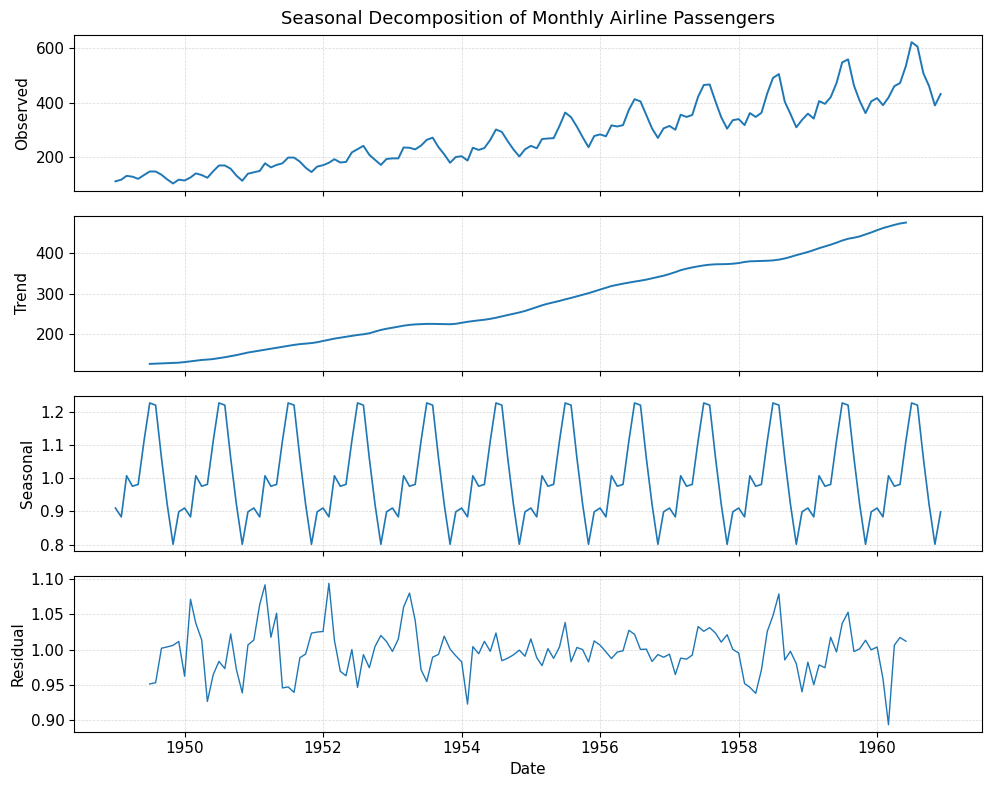
result = seasonal_decompose(ts, model="multiplicative", period=12)
So far this is standard. Now let’s make the figure nicer.
4. Academic-style plot
import matplotlib.pyplot as plt

plt.rcParams["figure.figsize"] = (10, 8)
plt.rcParams["font.size"] = 11

fig, axes = plt.subplots(4, 1, sharex=True)

# observed
axes[0].plot(result.observed, linewidth=1.4)
axes[0].set_ylabel("Observed")
axes[0].set_title("Seasonal Decomposition of Monthly Airline Passengers", fontsize=13, pad=8)

# trend
axes[1].plot(result.trend, linewidth=1.4)
axes[1].set_ylabel("Trend")

# seasonal
axes[2].plot(result.seasonal, linewidth=1.2)
axes[2].set_ylabel("Seasonal")

# residual
axes[3].plot(result.resid, linewidth=1.0)
axes[3].set_ylabel("Residual")
axes[3].set_xlabel("Date")

for ax in axes:
    ax.grid(True, linestyle="--", linewidth=0.5, alpha=0.5)

plt.tight_layout()
plt.show()
# fig.savefig("flights_decomposition.png", dpi=300, bbox_inches="tight")
At this point, most blogs stop here.
But since we're teaching this, we should answer the real question ⬇️
5. How are these components actually computed?
Let’s look at the classical (moving-average) decomposition idea first — this is roughly what seasonal_decompose is doing.
We assume:
- the data is equally spaced (monthly),
- the seasonal pattern has a known period (here 12),
- we can smooth out high-frequency fluctuations to get a trend.
We’ll explain it in the additive case first, because the logic is clearer. The multiplicative version is just “do the same thing on the log scale or by division.”
5.1 Step 1: Estimate the trend $T_t$
We want a smooth version of the series — no month-to-month noise, just the slow movement.
Classical way: centered moving average over one full season.
For a general centered moving average of odd length $m = 2k+1$:
$$
\hat{T}_t = \frac{1}{m} \sum_{i = -k}^{k} y_{t+i}, \quad \text{where } m = 2k+1
$$
For monthly data ($m=12$), a two-step centered moving average is often used.
If the period is even (like 12), we do a 2-step centering, but the idea is the same: average over one whole year to remove the within-year seasonality.
Intuition to tell students:
“If I average all 12 months around this point, the ‘January is high / February is low’ effect will cancel out, and I’m left with the slow trend.”
That gives us $\hat{T}_t$.
5.2 Step 2: Remove the trend to expose the seasonal part
Now we want to see “how much above/below the trend” each month is.
- Additive case:
$$
d_t = y_t - \hat{T}_t
$$ - Multiplicative case:
$$
d_t = \frac{y_t}{\hat{T}_t}
$$
This new series $d_t$ should mainly contain seasonality + small noise.
5.3 Step 3: Average by season (month)
Seasonality is repeating. That means:
- All Januaries should have a similar seasonal effect,
- All Februaries should have a similar seasonal effect,
- …
So we group by month and average:
- Additive:
$$
\hat{S}_{\text{Jan}} = \text{average of } d_t \text{ for all Januaries}
$$
$$
\hat{S}{\text{Feb}} = \text{average of } d_t \text{ for all Februaries}
$$
- Multiplicative:
$$
\hat{S}_{\text{Jan}} = \text{average of } \frac{y_t}{\hat{T}_t} \text{ for all Januaries}
$$
This gives us one seasonal number per month. Then we repeat this 12-number pattern over the whole timeline to create the seasonal series $\hat{S}_t$.
Sometimes we re-scale the seasonal factors so they sum to 0 (additive) or product to 1 (multiplicative), to make the decomposition “balanced”.
5.4 Step 4: Residual = whatever is left
Now we have:
- observed $y_t$,
- trend $\hat{T}_t$,
- seasonal $\hat{S}_t$.
So the residual / irregular is just:
- Additive:
$$
\hat{R}_t = y_t - \hat{T}_t - \hat{S}_t
$$ - Multiplicative:
$$
\hat{R}_t = \frac{y_t}{\hat{T}_t \times \hat{S}_t}
$$
That’s the “leftover” — the part the model can’t explain with smooth movement and repeating pattern.
You can literally say in class:
“Decomposition is ‘trend by smoothing’ + ‘seasonality by grouping’ + ‘residual by subtraction’.”
That sentence alone makes it non-mysterious for students.
6. What about STL?
Classical decomposition is nice and simple, but it has some limitations:
- trend is tied to that fixed moving-average window,
- seasonality is assumed to be very stable,
- outliers can disturb everything.
STL (Seasonal-Trend decomposition using Loess) fixes that by iteratively estimating:
- a smooth trend (with LOESS),
- a flexible seasonal component,
- optionally doing it in a robust way (down-weight outliers).
Code:
from statsmodels.tsa.seasonal import STL

stl = STL(ts, period=12, robust=True)
res = stl.fit()
fig = res.plot()
plt.show()
How to explain it shortly:
“Classical decomposition: fixed window + average by month.
STL: learn the shape of the season and the trend more flexibly.”
For research / messy operational data, STL is often the better choice.
7. Additive vs multiplicative (with flights)
Because the flights data’s seasonal fluctuations grow together with the level, the multiplicative model is more realistic:
from statsmodels.tsa.seasonal import seasonal_decompose

res_add = seasonal_decompose(ts, model="additive", period=12)
res_mul = seasonal_decompose(ts, model="multiplicative", period=12)
Tell students:
- Additive → seasonal effect is like “+10, +20, -5” every year
- Multiplicative → seasonal effect is like “×1.1, ×0.9, ×1.05” every year
Flights → multiplicative wins.
8. Why this matters
Once students understand how the components are obtained, they also understand:
- Why frequency matters → if you don’t tell the model it’s monthly (
period=12), it can’t group by month. - Why missing data is a problem → moving averages and group-by-month need complete data.
- Why decomposition helps forecasting → if seasonality is strong and stable, use a seasonal model.
- Why residuals are useful → detect anomalies on the part that should be random.
9. Full code in one place
import pandas as pd
import seaborn as sns
import matplotlib.pyplot as plt
from statsmodels.tsa.seasonal import seasonal_decompose

# load dataset
flights = sns.load_dataset("flights")
flights["date"] = pd.to_datetime(
    flights["year"].astype(str) + "-" + flights["month"].astype(str) + "-01"
)
ts = flights.set_index("date")["passengers"].asfreq("MS")

# decompose
result = seasonal_decompose(ts, model="multiplicative", period=12)

# plot nicely
plt.rcParams["figure.figsize"] = (10, 8)
plt.rcParams["font.size"] = 11

fig, axes = plt.subplots(4, 1, sharex=True)

axes[0].plot(result.observed, linewidth=1.4)
axes[0].set_ylabel("Observed")
axes[0].set_title("Seasonal Decomposition of Monthly Airline Passengers", fontsize=13, pad=8)

axes[1].plot(result.trend, linewidth=1.4)
axes[1].set_ylabel("Trend")

axes[2].plot(result.seasonal, linewidth=1.2)
axes[2].set_ylabel("Seasonal")

axes[3].plot(result.resid, linewidth=1.0)
axes[3].set_ylabel("Residual")
axes[3].set_xlabel("Date")

for ax in axes:
    ax.grid(True, linestyle="--", linewidth=0.5, alpha=0.5)

plt.tight_layout()
plt.show()
10. Final takeaway
So, to answer the original “math” question:
- We smooth to get the trend;
- We group by period to get the seasonal pattern;
- We subtract/divide to get the residual;
- In multiplicative cases, we work in ratios instead of differences;
- STL is a more flexible, iterative version of the same idea.
Once students see that, decomposition stops being a black box — and they’re ready to move on to ARIMA, SARIMA, Prophet, or even to deseasonalize → feed into ML/DL models.